Distributed Data Parallel Training
Scaling Training Across Multiple Devices/Machines
Training modern machine learning models has become an increasingly demanding computational challenge. As models scale to hundreds of billions—or even trillions—of parameters and datasets grow to unprecedented sizes, single-device training approaches are no longer feasible. Consider GPT-4, with its estimated 1.8 trillion parameters: training such a model on a single GPU would take several millennia1.
To address these computational demands, engineers have developed sophisticated distributed training strategies. One such strategy is distributed data parallelism.
Distributed Data Parallelism
Data parallelism addresses the computational bottleneck in training by distributing batches of training data across multiple GPUs, with each device maintaining a complete copy of the model. This approach enables parallel processing of different data samples while keeping the model architecture intact, significantly reducing training time through increased throughput. Figure 1 illustrates the distributed data-parallel training approach.
Gradients are synchronized across devices after each minibatch's backward pass2, ensuring all devices have the same aggregate gradients before the weight update step. During this synchronization, each device's local gradients are combined, and the result is distributed back to all nodes, allowing them to update their model parameters consistently.
It's important to note that this strategy is viable only when the entire model can fit in the device's memory, which can become a critical constraint as model sizes grow. It's ideal for scenarios with large datasets and relatively smaller models (typically under a few billion parameters), making it a good choice for many computer vision tasks.
Additionally, when using distributed data parallelism for model training, one must consider that the effective batch size increases with the number of GPUs. This may require adjusting the learning rate and other hyperparameters to maintain model convergence.
Different algorithms and communication patterns can be used to perform gradient synchronization in data-parallel training. One popular approach is the ring all-reduce algorithm.
Ring All-Reduce Algorithm
The ring all-reduce is a communication algorithm that tries to efficiently solve the problem of combining data across multiple devices/machines.
In naive approaches, where all processors send their data to a single master node for reduction, the communication overhead grows linearly with the number of processors, creating a significant bottleneck that limits scaling. For example, with N devices each sending D bytes of data, the master node must receive and process N×D bytes of data while also becoming a network bottleneck as it handles N separate incoming communications.
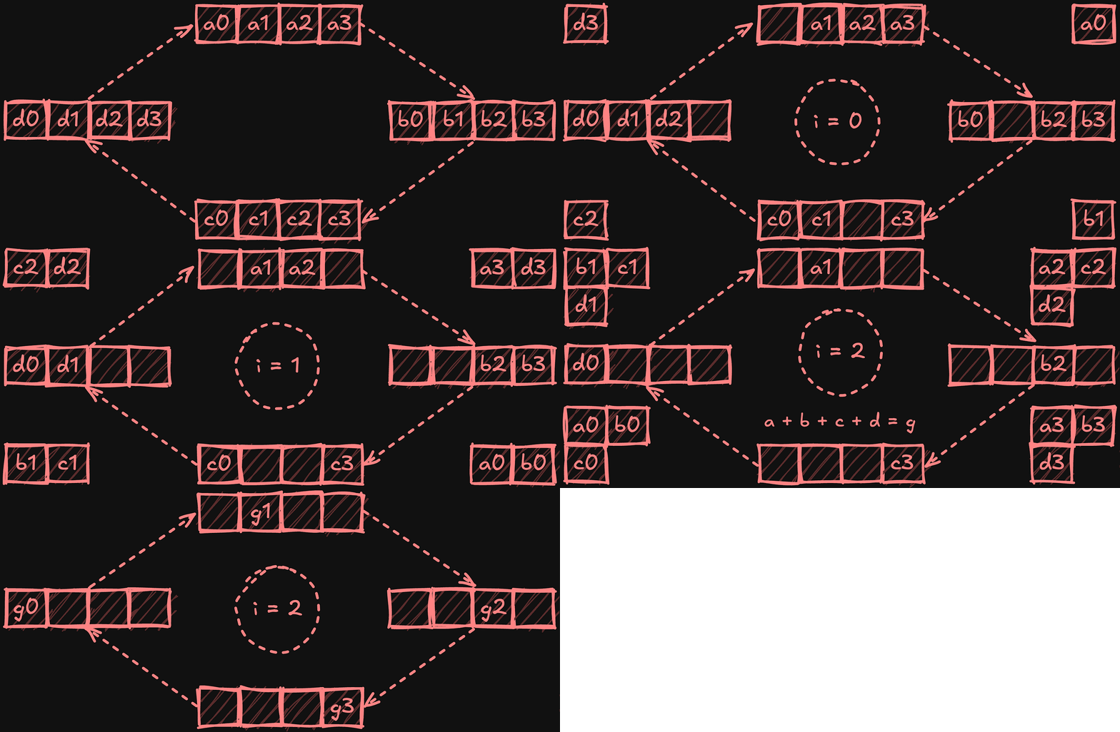
The ring all-reduce algorithm arranges processors in a logical ring, where each only communicates with its immediate neighbours. The algorithm occurs in two phases: scatter-reduce and all-gather. During scatter-reduce, each device divides its local data into equal chunks (one per processor) and progressively shares and reduces these chunks as they travel around the ring. Starting with i = 0 and using circular chunk indexing, for a processor p, the steps can be defined as:
Send chunk p - i to processor p + 1.
Receive chunk p - i - 1 and reduce with local chunk.
Increment i and repeat while i < p - 1.
At the end of this phase, each processor holds a fully reduced chunk.
In the subsequent all-gather phase, processors circulate these reduced chunks around the ring, with each processor collecting a copy of each chunk. After N-1 steps (where N is the number of processors), every processor obtains a complete copy of the fully reduced chunks.
The total data transferred in ring all-reduce can be expressed as:
The formula reflects the algorithm's two-phase structure: N-1 steps for scatter-reduce and N-1 steps for all-gather, giving us the 2(N-1) factor. In each step, devices communicate chunks of size K/N, as the original data of size K is divided into N equal parts.
This formula simplifies to 2K, showing that the transferred data remains constant regardless of the number of processors. Given optimal GPU topology arrangement, the algorithm achieves bandwidth optimality when latency costs are negligible compared to bandwidth constraints.
Ring All-Reduce in Deep Learning
In deep learning, ring all-reduce enables efficient gradient synchronization during distributed training across multiple GPUs or compute nodes. During each training iteration, each GPU computes gradients for its local data batch, and these gradients must be averaged across all devices to maintain model consistency.
Ring all-reduce performs best when GPUs within the same node are placed adjacent to each other in the ring, minimizing network contention. Since data transfers happen synchronously between neighbours, the algorithm's speed is limited by the slowest connection in the ring.
Further performance gains come from exploiting the neural network's layer-wise structure: during each iteration, while GPUs perform forward propagation for error computation followed by backpropagation for gradient calculation, gradients become available sequentially from the output layer inward. Since ring all-reduce can operate on parameter subsets, we can begin reducing output layer gradients while earlier layers are still computing their gradients. This interleaving of communication and computation significantly reduces GPU idle time during synchronization.
As an example, PyTorch's distributed training in Kubernetes via the Kubeflow training operator utilizes ring all-reduce.
Latency of Ring All-Reduce
For large distributed systems, latency isn’t negligible. While ring all-reduce achieves optimal bandwidth utilization under ideal conditions, its latency profile creates scaling limitations. For each synchronization round, the algorithm must perform 2(N-1) sequential communication steps, where N represents the number of participating processors. This creates a linear relationship between latency and processor count that becomes challenging in large-scale training clusters. Given how computationally expensive network operations are, the cumulative effect of these communication steps can substantially impact overall training performance as more GPUs or nodes join the cluster.
Tree All-Reduce
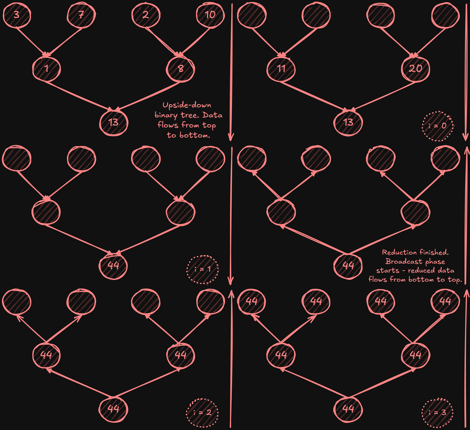
The tree all-reduce is a distributed algorithm that uses a binary tree topology to combine data across multiple nodes efficiently (latency-wise). Picture an upside-down binary tree: Nodes at the top send data down to their parent nodes, which combine the received values. The process takes log2(N) steps, making its latency dramatically lower than ring all-reduce’s N steps - with 1024 nodes, tree all-reduce completes in just 10 communication steps versus ring reduce's 1024 steps. Here's how it works:
Reduce phase:
Leaf nodes send their values to their parent nodes.
Parent nodes combine received values and send to their parents.
This continues until root node performs final reduction.
Broadcast phase:
Root node sends result to its two children.
Each parent broadcasts received value to its two children.
Process continues until reaching leaf nodes.
Total latency is 2*log2(N) steps - log2(N) for reduce, log2(N) for broadcast.
The key limitation is in bandwidth utilization—leaf nodes, which constitute half of all nodes, use their network links in a half-duplex manner. Although they send data during the reduce phase and receive data during the broadcast phase, they never fully leverage their full-duplex capacity at any single point in time. While pipelining can help internal nodes overlap sending and receiving operations, it doesn’t address the fact that leaf nodes alternate between sending and receiving, rather than performing both simultaneously, thus leaving potential bandwidth underutilized.
Two-Tree All-Reduce
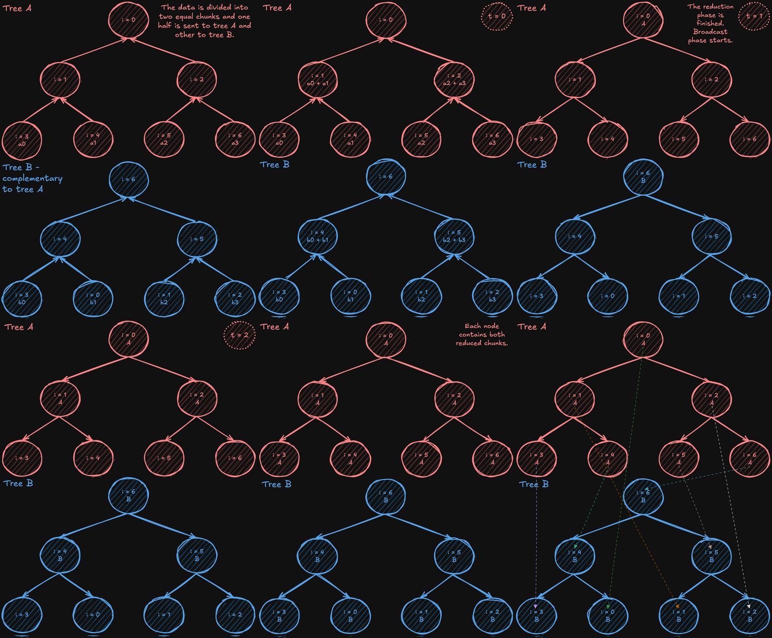
Two-tree all-reduce is an algorithm (introduced by Sanders, Traff, and Larsson in 2009) that tackles the bandwidth underutilization in simple tree reductions by starting with a complete (but not necessarily full) binary tree and then constructing a complementary one. In one tree, a node acts as a leaf; in the other, it becomes an internal node. By “shifting” or “mirroring” the numbering from the original complete tree to form the second tree, the internal nodes of one tree align with the leaves of the other, creating a perfectly interwoven communication pattern.
After constructing these two complementary trees, the data is split into two halves. Except for the initial steps (when the data is being first sent) and the final steps (when the last pieces of data are delivered), each intermediate communication phase allows every processor to both send and receive simultaneously, nearly doubling the effective bandwidth usage compared to a single-tree approach. While not every stage can perfectly utilize all bandwidth due to these startup and wind-down phases, the vast majority of steps achieve full-duplex efficiency. At the same time, the algorithm still operates in a logarithmic number of steps, like a standard tree all-reduce, maintaining low latency overall.
The two-tree all-reduce combines the O(logN) latency advantages of tree-based methods with high-bandwidth efficiency, making it an attractive algorithm for large-scale distributed training environments.
Performance Impact
In 2019, NVIDIA published the article “Massively Scale Your Deep Learning Training with NCCL 2.4,” which examined how different all-reduce algorithms—ring all-reduce, hierarchical ring all-reduce, and two-tree all-reduce—impact performance. Their findings are summarized below:


Conclusions
As modern machine learning models and datasets continue to expand, single-device training quickly becomes impractical, demanding distributed strategies like data parallelism to harness multiple GPUs. In such scenarios, communication overhead emerges as an important factor, with both bandwidth utilization and latency playing pivotal roles in training efficiency. For gradient synchronization, algorithms like the two-tree all-reduce combine the low-latency strengths of tree-based methods with near-full bandwidth utilization, providing an appealing, scalable solution for large-scale model training.
Based on community estimates, GPT-4's training reportedly utilized a cluster of 20,000-25,000 NVIDIA A100 GPUs over 3-4 months. To put this in perspective, if the same training were attempted on a single A100 GPU (assuming linear scaling), it would take between 5,000 to 8,300 years to complete.
As we cover later in this article, more efficient strategies initiate gradient synchronization as soon as partial gradients are ready, overlapping communication with computation and reducing GPU idle time.


